MicroPheno
MicroPheno’s paper is still under review. Please cite the bioarXiv version: Asgari E, Garakani K, McHardy AC and Mofrad MRK (2018)
MicroPheno: Predicting environments and host phenotypes from 16S rRNA gene sequencing using a k-mer based representation of shallow sub-samples. bioRxiv.
Available at: https://www.biorxiv.org/content/early/2018/01/28/255018.
The implementation is available at Contact: Ehsaneddin Asgari (asgari [at] berkeley [dot] edu) The processed datasets used in the paper are also available for download.
Summary
Motivation: Microbial communities play important roles in the function and maintenance of various biosystems, ranging from the human body to the environment. A major challenge in microbiome research is the classification of microbial communities of different environments or host phenotypes. The most common and cost-effective approach for such studies to date is 16S rRNA gene sequencing. Recent falls in sequencing costs have increased the demand for simple, efficient, and accurate methods for rapid detection or diagnosis with proved applications in medicine, agriculture, and forensic science. We describe a reference- and alignment-free approach for predicting environments and host phenotypes from 16S rRNA gene sequencing based on k-mer representations that benefits from a bootstrapping framework for investigating the sufficiency of shallow sub-samples. Deep learning methods as well as classical approaches were explored for predicting environments and host phenotypes. Results: k-mer distribution of shallow sub-samples outperformed the computationally costly Operational Taxonomic Unit (OTU) features in the tasks of body-site identification and Crohn’s disease prediction. Aside from being more accurate, using k-mer features in shallow sub-samples allows (i) skipping computationally costly sequence alignments required in OTU-picking, and (ii) provided a proof of concept for the sufficiency of shallow and short-length 16S rRNA sequencing for phenotype prediction. In addition, k-mer features predicted representative 16S rRNA gene sequences of 18 ecological environments, and 5 organismal environments with high macro-F1 scores of 0.88 and 0.87. For large datasets, deep learning outperformed classical methods such as Random Forest and SVM.
|
||||||||||||||||||||||||
Installation
MicroPheno is implemented in Python3.x and uses ScikitLearn and Keras frameworks for machine learning. To install the dependencies use the following command:
pip install -r requirements.txtPlease cite the MicroPheno ![]()
![]() .
.
User Manual
MicroPheno can be used either via the templates provided in the ipython notebooks or the command-line interface.
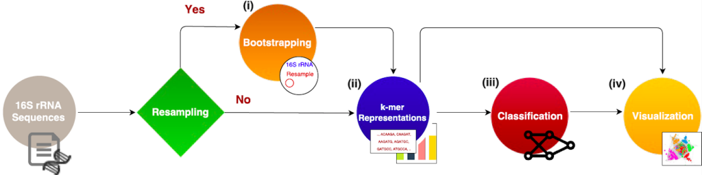
Bootstrapping
An example of bootstrapping provided in the notebooks.
Command line use: Argument to be used are the input/output directories, the sequence filetype, the k-mers and the sample size. Use argument ‘-h’ to see the helpers.
python3 micropheno.py --bootstrap --indir /path/to/16srRNAsamples/ --out output_dir/ --filetype fastq --kvals 3,4,5,6 --nvals 10,100,200,500,1000 --name crohsThe output would be generating the following plot in the specified output directory. See the related notebook for more details.

Representation Creation
Two examples of representation creation are provided in the notebooks, one with sampling from sequence files and the other for mapping the representative sequences.
Command line use: Argument to be used are the input/output directories, the sequence filetype, the k-mers and their sample size as well as number of cores to be used. Use argument ‘-h’ to see the helpers.
python3 micropheno.py --genkmer --inaddr /path/to/16srRNAsamples/ --out output_dir/ --filetype fastq --cores 20 --KN 6:100,6:1000,2:100 --name test_crohnClassification with Random Forest and SVM
The trained representation in the previous step in the input for classification.
See an example in the notebooks.
Command line use: Argument to be used are the X and Y, the classification algorithm (SVM, or RF), output directory as well as number of cores to be used. Use argument ‘-h’ to see the helpers.
The following command will do tuning the parameters as well as evaluation within a 10xFold corss-validation scheme. Details on how to parse the results (scores, confusion matrix, best estimator, etc) are provided here.
python3 micropheno.py --train_predictor --model RF (or SVM) --x k-mer.npz --y labels_phenotypes.txt --cores 20 --name test_crohn --out output_dir/Classification with Deep Neural Network
We use the Multi-Layer-Perceptrons (MLP) Neural Network architecture with several hidden layers using Rectified Linear Unit (ReLU) as the nonlinear activation function. We use softmax activation function at the last layer to produce the probability vector that can be regarded as representing posterior probabilities (Goodfellow-et-al-2016). To avoid overfitting we perform early stopping and also use dropout at hidden layers (Srivastava2014). A schematic visualization of our Neural Networks is depicted in the Figure.

Our objective is minimizing the loss, i.e. cross entropy between output and the one-hot vector representation of the target class. The error (the distance between the output and the target) is used to update the network parameters via a Back-propagation algorithm using Adaptive Moment Estimation (Adam) as optimizer (Kingma2015).
You can see an example in the notebooks here, showing how to see the learning curves and also getting the activation function of the neural network from the trained model.
Command line use: Argument to be used are the X and Y, the DNN flag, the neural network architecture (hidden-sizes and dropouts), batch size, number of epochs, output directory as well as the GPU id to be used. Use argument ‘-h’ to see the helpers.
python3 micropheno.py --train_predictor --model DNN --arch --batchsize 10 --epochs 100 --x k-mer.npz --y labels_phenotypes.txt --name test_crohn --out output_dir/Visualization
An example of visualization using PCA, t-SNE, as well as t-SNE over the activation function of the last layer of the neural network is provided in this notebook.
